Partial derivative: CH:5 IN ENGINEERING
In mathematics, a partial derivative of a function of several variables is its derivative with respect to one of those variables, with the others held constant (as opposed to the total derivative, in which all variables are allowed to vary). Partial derivatives are used in vector calculus and differential geometry.
The partial derivative of a function f with respect to the variable x is variously denoted by

Introduction:
Suppose that ƒ is a function of more than one variable. For instance,
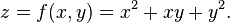
The graph of this function defines a surface in Euclidean space. To every point on this surface, there are an infinite number of tangent lines. Partial differentiation is the act of choosing one of these lines and finding its slope. Usually, the lines of most interest are those that are parallel to the xz-plane, and those that are parallel to the yz-plane (which result from holding either y or x constant, respectively.)
To find the slope of the line tangent to the function at P(1, 1, 3) that is parallel to the xz-plane, the y variable is treated as constant. The graph and this plane are shown on the right. On the graph below it, we see the way the function looks on the plane y = 1. By finding the derivative of the equation while assuming that y is a constant, the slope of ƒ at the point (x, y, z) is found to be:


Definition:
Basic definition,
The function f can be reinterpreted as a family of functions of one variable indexed by the other variables:


In general, the partial derivative of a function f(x1,...,xn) in the direction xi at the point (a1,...,an) is defined to be:

 , and by definition,
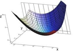
An important example of a function of several variables is the case of a scalar-valued function f(x1,...xn) on a domain in Euclidean space Rn (e.g., on R2 or R3). In this case f has a partial derivative ∂f/∂xj with respect to each variable xj. At the point a, these partial derivatives define the vector
A common abuse of notation is to define the del operator (∇) as follows in three-dimensional Euclidean space R3 with unit vectors
 :
:![\nabla = \bigg[{\frac{\partial}{\partial x}} \bigg] \mathbf{\hat{i}} + \bigg[{\frac{\partial}{\partial y}}\bigg] \mathbf{\hat{j}} + \bigg[{\frac{\partial}{\partial z}}\bigg] \mathbf{\hat{k}}](http://upload.wikimedia.org/math/f/e/4/fe4954365d1dc12dbbc804b923dfdae3.png)
 ):
):![\nabla = \sum_{j=1}^n \bigg[{\frac{\partial}{\partial x_j}}\bigg] \mathbf{\hat{e}_j} = \bigg[{\frac{\partial}{\partial x_1}}\bigg] \mathbf{\hat{e}_1} + \bigg[{\frac{\partial}{\partial x_2}}\bigg] \mathbf{\hat{e}_2} + \bigg[{\frac{\partial}{\partial x_3}}\bigg] \mathbf{\hat{e}_3} + \dots + \bigg[{\frac{\partial}{\partial x_n}}\bigg] \mathbf{\hat{e}_n}](http://upload.wikimedia.org/math/0/8/b/08b7a94d4e192df78103570d96fcd1c3.png)
Formal definition
Like ordinary derivatives, the partial derivative is defined as a limit. Let U be an open subset of Rn and f : U → R a function. The partial derivative of f at the point a = (a1, ..., an) ∈ U with respect to the i-th variable ai is defined as
The partial derivative
 can be seen as another function defined on U
and can again be partially differentiated. If all mixed second order
partial derivatives are continuous at a point (or on a set), f is termed a C2 function at that point (or on that set); in this case, the partial derivatives can be exchanged by Clairaut's theorem:
can be seen as another function defined on U
and can again be partially differentiated. If all mixed second order
partial derivatives are continuous at a point (or on a set), f is termed a C2 function at that point (or on that set); in this case, the partial derivatives can be exchanged by Clairaut's theorem:
Examples:
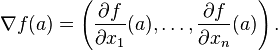
The volume V of a cone depends on the cone's height h and its radius r according to the formula


By contrast, the total derivative of V with respect to r and h are respectively


If (for some arbitrary reason) the cone's proportions have to stay the same, and the height and radius are in a fixed ratio k,


Notation:
For the following examples, let f be a function in x, y and z.First-order partial derivatives:


Antiderivative analogue:
There is a concept for partial derivatives that is analogous to antiderivatives for regular derivatives. Given a partial derivative, it allows for the partial recovery of the original function.
Consider the example of . The "partial" integral can be taken with respect to x (treating y as constant, in a similar manner to partial derivation):

 will disappear when taking the partial derivative, and we have to
account for this when we take the antiderivative. The most general way
to represent this is to have the "constant" represent an unknown
function of all the other variables.
will disappear when taking the partial derivative, and we have to
account for this when we take the antiderivative. The most general way
to represent this is to have the "constant" represent an unknown
function of all the other variables.Thus the set of functions
 , where g is any one-argument function, represents the entire set of functions in variables x,y that could have produced the x-partial derivative 2x+y.
If all the partial derivatives of a function are known (for example, with the gradient), then the antiderivatives can be matched via the above process to reconstruct the original function up to a constant
")
")
")
")
")
")
")
")


